Nearest Neighbor Adjustment of Predictions

For regression models (i.e., predicting numeric outcomes), this function compares a predicted value to the predictions from the training set and uses their values to increase or decrease the original prediction.

nn_adjust(wflow, training, ...)

# S3 method for default
nn_adjust(wflow, training, ...)

# S3 method for workflow
nn_adjust(wflow, training, butcher = FALSE, ...)

Arguments

wflow: A fitted workflows::workflow() object.
training: A data frame containing the predictors and outcome data used to create wflow.
...: Not currently used.
butcher: A logical: should butcher::butcher() be used to trim the workflow's size?

Value

An object of class nn_adjust. It contains the training set, fitted workflow, and other details.

Details

Gower’s method finds the K training set points that are most similar to the sample being predicted. This distance method is appropriate for qualitative and quantitative predictors and does not require normalization.

For the $i=1\ldots K$ nearest neighbors, the method computes the adjusted predicted value based on

$$\widehat{a}^*_i = y_i + ( \widehat{y}_{new} - \widehat{y}_i)$$

then takes a weighted mean as the final predicted value. The weights are the inverse of the Gower distance plus a small constant (defaulted to 0.5 but is changeable).

The number of neighbors does not need to be declared until the adjustment is executed by predict.nn_adjust() or augment.nn_adjust().

References

Quinlan R (1993). "Combining instance–based and model–based learning." Proceedings of the Tenth International Conference on Machine Learning, pp. 236-243. Gower, J (1971). "A general coefficient of similarity and some of its properties." Biometrics, pp. 857-871.

Examples

if (rlang::is_installed(c("ggplot2", "parsnip", "rpart", "MASS"))) {

  library(workflows)
  library(dplyr)
  library(parsnip)
  library(ggplot2)

  # ------------------------------------------------------------------------------
  # Use the 1D motorcycle helmet data as an example

  data(mcycle, package = "MASS")

  # Use every fifth data point as a test point
  in_test <- ( 1:nrow(mcycle) ) %% 5 == 0
  cycl_train <- mcycle[-in_test, ]
  cycl_test  <- mcycle[ in_test, ]

  # A grid to show the predicted lines
  mcycle_grid <- tibble(times = seq(2.4, 58, length.out = 500))

  # ------------------------------------------------------------------------------
  # Fit a decision tree

  cart_spec <- decision_tree() %>% set_mode("regression")

  cart_fit <-
    workflow(accel ~ times, cart_spec) %>%
    fit(data = cycl_train)

  raw_pred <- augment(cart_fit, mcycle_grid)

  raw_pred %>%
    ggplot(aes(x = times)) +
    geom_point(data = cycl_test, aes(y = accel)) +
    geom_line(aes(y = .pred),  col = "blue", alpha = 3 / 4) +
    theme_bw()

  # ------------------------------------------------------------------------------
  # Get adjusted predictions

  adj_obj <- nn_adjust(cart_fit, cycl_train)
  adj_pred <- augment(adj_obj, mcycle_grid, neighbors = 10)

  adj_pred %>%
    ggplot(aes(x = times)) +
    geom_point(data = cycl_test, aes(y = accel)) +
    geom_line(aes(y = .pred),  col = "orange", alpha = 3 / 4) +
    theme_bw()

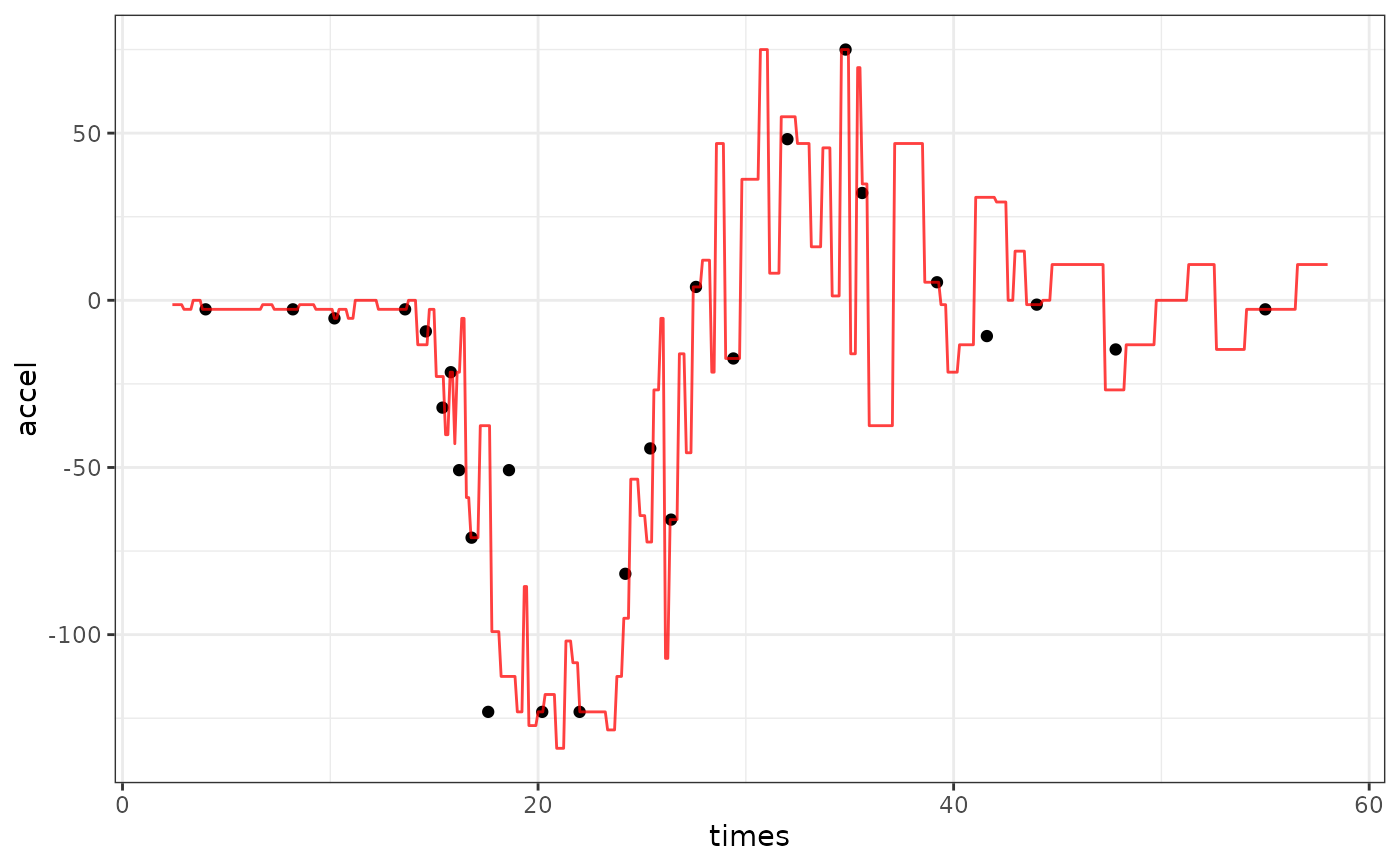
  # 1 neighbor is usually pretty bad

  adj_pred_1 <- augment(adj_obj, mcycle_grid, neighbors = 1)

  adj_pred_1 %>%
    ggplot(aes(x = times)) +
    geom_point(data = cycl_test, aes(y = accel)) +
    geom_line(aes(y = .pred),  col = "red", alpha = 3 / 4) +
    theme_bw()

}