library(tidymodels)
#> ── Attaching packages ────────────────────────────────────── tidymodels 1.2.0 ──
#> ✔ broom        1.0.5          ✔ recipes      1.0.10
#> ✔ dials        1.2.1          ✔ rsample      1.2.0
#> ✔ dplyr        1.1.4          ✔ tibble       3.2.1
#> ✔ ggplot2      3.5.0          ✔ tidyr        1.3.1
#> ✔ infer        1.0.6          ✔ tune         1.2.0
#> ✔ modeldata    1.3.0          ✔ workflows    1.1.4
#> ✔ parsnip      1.2.1          ✔ workflowsets 1.1.0.9000
#> ✔ purrr        1.0.2          ✔ yardstick    1.3.1
#> ── Conflicts ───────────────────────────────────────── tidymodels_conflicts() ──
#> ✖ purrr::discard() masks scales::discard()
#> ✖ dplyr::filter()  masks stats::filter()
#> ✖ dplyr::lag()     masks stats::lag()
#> ✖ recipes::step()  masks stats::step()
#> • Dig deeper into tidy modeling with R at https://www.tmwr.org

tidymodels_prefer()Introduction to Machine Learning with tidymodels
Max Kuhn and Simon Couch
👋 Who am I?

![]()
![]()
![]()
👋 Who are we?


👋 Who are you?
Ypu have a good working knowledge of R, and be familiar with basic data wrangling and visualisation as described in R for Data Science by Wickham and Grolemund (2016).
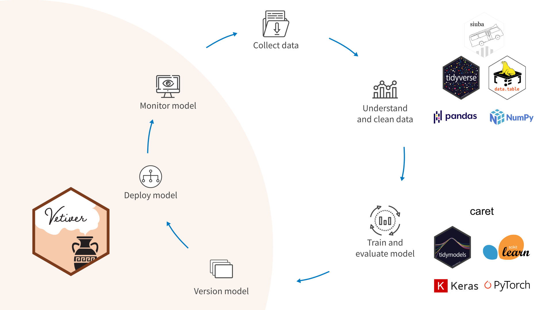
What is tidymodels?
The tidymodels framework is a collection of packages for modeling and machine learning using tidyverse principles.
- tidymodels.org
…so what is modeling and machine learning?
BYO Venn Diagram

The tidymodels framework is a collection of packages for safe, performant, and expressive supervised predictive modeling on tabular data.
🥴
The tidymodels framework is a collection of packages for safe, performant, and expressive supervised predictive modeling on tabular data.
🥴
The tidymodels framework is a collection of packages for safe, performant, and expressive supervised predictive modeling on tabular data.
🥴
The tidymodels framework is a collection of packages for safe, performant, and expressive supervised predictive modeling on tabular data.
🥴
The tidymodels framework is a collection of packages for safe, performant, and expressive supervised predictive modeling on tabular data.
🥴
Think about the modeling problem, not the syntax.
The Meta-package
Why tidymodels?
Why tidymodels? Consistency
How many different ways can you think of to fit a linear model in R?
The blessing:
- Many statistical modeling practitioners implement methods in R
The curse:
- Many statistical modeling practitioners implement methods in R
Why tidymodels? Consistency
mtcars
#>                      mpg cyl  disp  hp drat    wt  qsec vs am gear
#> Mazda RX4           21.0   6 160.0 110 3.90 2.620 16.46  0  1    4
#> Mazda RX4 Wag       21.0   6 160.0 110 3.90 2.875 17.02  0  1    4
#> Datsun 710          22.8   4 108.0  93 3.85 2.320 18.61  1  1    4
#> Hornet 4 Drive      21.4   6 258.0 110 3.08 3.215 19.44  1  0    3
#> Hornet Sportabout   18.7   8 360.0 175 3.15 3.440 17.02  0  0    3
#> Valiant             18.1   6 225.0 105 2.76 3.460 20.22  1  0    3
#> Duster 360          14.3   8 360.0 245 3.21 3.570 15.84  0  0    3
#> Merc 240D           24.4   4 146.7  62 3.69 3.190 20.00  1  0    4
#> Merc 230            22.8   4 140.8  95 3.92 3.150 22.90  1  0    4
#> Merc 280            19.2   6 167.6 123 3.92 3.440 18.30  1  0    4
#> Merc 280C           17.8   6 167.6 123 3.92 3.440 18.90  1  0    4
#> Merc 450SE          16.4   8 275.8 180 3.07 4.070 17.40  0  0    3
#> Merc 450SL          17.3   8 275.8 180 3.07 3.730 17.60  0  0    3
#> Merc 450SLC         15.2   8 275.8 180 3.07 3.780 18.00  0  0    3
#> Cadillac Fleetwood  10.4   8 472.0 205 2.93 5.250 17.98  0  0    3
#> Lincoln Continental 10.4   8 460.0 215 3.00 5.424 17.82  0  0    3
#> Chrysler Imperial   14.7   8 440.0 230 3.23 5.345 17.42  0  0    3
#> Fiat 128            32.4   4  78.7  66 4.08 2.200 19.47  1  1    4
#> Honda Civic         30.4   4  75.7  52 4.93 1.615 18.52  1  1    4
#> Toyota Corolla      33.9   4  71.1  65 4.22 1.835 19.90  1  1    4
#> Toyota Corona       21.5   4 120.1  97 3.70 2.465 20.01  1  0    3
#> Dodge Challenger    15.5   8 318.0 150 2.76 3.520 16.87  0  0    3
#> AMC Javelin         15.2   8 304.0 150 3.15 3.435 17.30  0  0    3
#> Camaro Z28          13.3   8 350.0 245 3.73 3.840 15.41  0  0    3
#> Pontiac Firebird    19.2   8 400.0 175 3.08 3.845 17.05  0  0    3
#> Fiat X1-9           27.3   4  79.0  66 4.08 1.935 18.90  1  1    4
#> Porsche 914-2       26.0   4 120.3  91 4.43 2.140 16.70  0  1    5
#> Lotus Europa        30.4   4  95.1 113 3.77 1.513 16.90  1  1    5
#> Ford Pantera L      15.8   8 351.0 264 4.22 3.170 14.50  0  1    5
#> Ferrari Dino        19.7   6 145.0 175 3.62 2.770 15.50  0  1    5
#> Maserati Bora       15.0   8 301.0 335 3.54 3.570 14.60  0  1    5
#> Volvo 142E          21.4   4 121.0 109 4.11 2.780 18.60  1  1    4
#>                     carb
#> Mazda RX4              4
#> Mazda RX4 Wag          4
#> Datsun 710             1
#> Hornet 4 Drive         1
#> Hornet Sportabout      2
#> Valiant                1
#> Duster 360             4
#> Merc 240D              2
#> Merc 230               2
#> Merc 280               4
#> Merc 280C              4
#> Merc 450SE             3
#> Merc 450SL             3
#> Merc 450SLC            3
#> Cadillac Fleetwood     4
#> Lincoln Continental    4
#> Chrysler Imperial      4
#> Fiat 128               1
#> Honda Civic            2
#> Toyota Corolla         1
#> Toyota Corona          1
#> Dodge Challenger       2
#> AMC Javelin            2
#> Camaro Z28             4
#> Pontiac Firebird       2
#> Fiat X1-9              1
#> Porsche 914-2          2
#> Lotus Europa           2
#> Ford Pantera L         4
#> Ferrari Dino           6
#> Maserati Bora          8
#> Volvo 142E             2
Why tidymodels? Consistency
Why tidymodels? Consistency
Why tidymodels? Consistency
Why tidymodels? Consistency
Why tidymodels? Safety1
Why tidymodels? Safety1
- Overfitting leads to analysts believing models are more performant than they actually are.
- A 2023 review found data leakage to be “a widespread failure mode in machine-learning (ML)-based science.”
- Implementations of the same machine learning model give differing results, resulting in irreproducibility of modeling results.
Why tidymodels? Safety
Some of the resistance I’ve seen to tidymodels comes from a place of “This makes it too easy- you’re not thinking carefully about what the code is doing!” But I think this is getting it backwards.
By removing the burden of writing procedural logic, I get to focus on scientific and statistical questions about my data and model.
Why tidymodels? Completeness

Why tidymodels? Completeness
Built-in support for 99 machine learning models!
#> # A tibble: 99 × 2
#>    name       engine
#>    <chr>      <chr>
#>  1 boost_tree C5.0
#>  2 boost_tree h2o
#>  3 boost_tree h2o_gbm
#>  4 boost_tree lightgbm
#>  5 boost_tree mboost
#>  6 boost_tree spark
#>  7 boost_tree xgboost
#>  8 null_model parsnip
#>  9 svm_linear LiblineaR
#> 10 svm_linear kernlab
#> # ℹ 89 more rows
Why tidymodels? Completeness
Built-in support for 102 data pre-processing techniques!
#> # A tibble: 102 × 1
#>    name
#>    <chr>
#>  1 step_rename_at
#>  2 step_scale
#>  3 step_kpca
#>  4 step_percentile
#>  5 step_depth
#>  6 step_poly_bernstein
#>  7 step_impute_linear
#>  8 step_novel
#>  9 step_nnmf_sparse
#> 10 step_slice
#> # ℹ 92 more rows
Why tidymodels? Extensibility
Can’t find the technique you need?

Why tidymodels? Extensibility
Why tidymodels? Deployability
Tightly integrated with Posit Workbench and Connect
- Workbench: scalable, on-demand computational resources
- Connect: share work with collaborators and practitioners
The vetiver package makes it extremely easy to publish your model.
Applied example 🍕🍕
Food deliveries
These data are in the modeldata package.
glimpse(deliveries)
#> Rows: 10,012
#> Columns: 31
#> $ time_to_delivery <dbl> 16.1106, 22.9466, 30.2882, 33.4266, 27.2255…
#> $ hour             <dbl> 11.899, 19.230, 18.374, 15.836, 19.619, 12.…
#> $ day              <fct> Thu, Tue, Fri, Thu, Fri, Sat, Sun, Thu, Fri…
#> $ distance         <dbl> 3.15, 3.69, 2.06, 5.97, 2.52, 3.35, 2.46, 2…
#> $ item_01          <int> 0, 0, 0, 0, 0, 1, 0, 0, 0, 0, 0, 0, 0, 1, 0…
#> $ item_02          <int> 0, 0, 0, 0, 0, 0, 0, 0, 0, 2, 0, 0, 0, 1, 0…
#> $ item_03          <int> 2, 0, 0, 0, 0, 0, 1, 1, 0, 1, 0, 0, 0, 0, 1…
#> $ item_04          <int> 0, 0, 0, 0, 1, 1, 1, 0, 0, 0, 1, 0, 1, 0, 0…
#> $ item_05          <int> 0, 0, 1, 0, 0, 0, 0, 0, 0, 0, 0, 0, 0, 0, 0…
#> $ item_06          <int> 0, 0, 0, 0, 0, 0, 0, 1, 0, 0, 0, 0, 0, 0, 0…
#> $ item_07          <int> 0, 0, 0, 0, 1, 1, 0, 0, 1, 0, 0, 0, 0, 0, 0…
#> $ item_08          <int> 0, 0, 0, 0, 0, 0, 0, 1, 0, 0, 1, 0, 1, 0, 0…
#> $ item_09          <int> 0, 0, 0, 0, 0, 1, 0, 0, 0, 0, 0, 0, 1, 0, 1…
#> $ item_10          <int> 1, 0, 0, 0, 0, 0, 0, 0, 0, 0, 0, 1, 0, 0, 0…
#> $ item_11          <int> 1, 0, 0, 0, 1, 1, 0, 0, 0, 0, 0, 0, 0, 0, 0…
#> $ item_12          <int> 0, 0, 0, 1, 0, 0, 0, 0, 0, 1, 0, 0, 0, 0, 0…
#> $ item_13          <int> 0, 0, 0, 0, 0, 0, 0, 0, 0, 0, 0, 0, 0, 0, 0…
#> $ item_14          <int> 0, 0, 0, 0, 1, 0, 0, 0, 0, 0, 0, 0, 0, 0, 0…
#> $ item_15          <int> 0, 0, 0, 0, 0, 0, 0, 0, 1, 0, 0, 0, 0, 0, 0…
#> $ item_16          <int> 0, 0, 0, 0, 0, 0, 0, 0, 0, 0, 0, 0, 0, 0, 0…
#> $ item_17          <int> 0, 0, 0, 0, 0, 0, 0, 0, 0, 1, 0, 0, 0, 0, 0…
#> $ item_18          <int> 0, 1, 0, 0, 0, 0, 0, 0, 0, 1, 0, 0, 0, 0, 0…
#> $ item_19          <int> 0, 0, 0, 0, 0, 0, 0, 0, 0, 0, 0, 0, 0, 0, 0…
#> $ item_20          <int> 0, 0, 1, 0, 0, 0, 0, 0, 0, 0, 0, 0, 0, 0, 0…
#> $ item_21          <int> 0, 0, 0, 0, 0, 0, 0, 1, 0, 0, 0, 0, 0, 0, 0…
#> $ item_22          <int> 0, 0, 0, 0, 0, 1, 1, 0, 0, 1, 0, 0, 0, 1, 0…
#> $ item_23          <int> 0, 0, 0, 0, 0, 0, 0, 0, 0, 0, 0, 0, 0, 0, 0…
#> $ item_24          <int> 0, 0, 1, 0, 0, 1, 0, 0, 0, 0, 0, 0, 0, 0, 0…
#> $ item_25          <int> 0, 0, 0, 0, 0, 0, 0, 0, 0, 0, 1, 0, 0, 0, 0…
#> $ item_26          <int> 0, 0, 0, 0, 0, 0, 0, 0, 1, 0, 0, 1, 0, 0, 0…
#> $ item_27          <int> 0, 0, 0, 1, 1, 0, 0, 0, 0, 0, 0, 1, 1, 0, 0…
Investigate the data!
Let’s take 10m and have you explore the data.
Let me know what you think about them. (not a trick question)
10:00 Splitting the data
We typically start by splitting the data into partitions used for modeling and assessment:
Splitting the data (with validation)
Instead, let’s do a 3-way split to include a validation set that we can use before the test set:
(TMwR)
A linear model
mod_spec <- linear_reg()
mod_fit <- mod_spec %>% fit(time_to_delivery ~ ., data = delivery_train)

tidy(mod_fit)
#> # A tibble: 36 × 5
#>    term        estimate std.error statistic   p.value
#>    <chr>          <dbl>     <dbl>     <dbl>     <dbl>
#>  1 (Intercept)   -18.4     0.372     -49.4  0
#>  2 hour            1.78    0.0169    105.   0
#>  3 dayTue          1.02    0.254       4.02 5.77e-  5
#>  4 dayWed          3.46    0.230      15.1  9.52e- 51
#>  5 dayThu          5.04    0.225      22.4  9.71e-108
#>  6 dayFri          6.98    0.220      31.7  1.49e-207
#>  7 daySat          7.82    0.219      35.7  2.81e-259
#>  8 daySun          3.53    0.229      15.4  5.15e- 53
#>  9 distance        2.78    0.0414     67.0  0
#> 10 item_01         1.61    0.140      11.5  2.13e- 30
#> # ℹ 26 more rows
A linear model
# Good:
predict(mod_fit, head(delivery_val, 3))
#> # A tibble: 3 × 1
#>   .pred
#>   <dbl>
#> 1  12.4
#> 2  27.2
#> 3  20.2

# Better:
augment(mod_fit, head(delivery_val, 3)) %>% select(1:9)
#> # A tibble: 3 × 9
#>   .pred .resid time_to_delivery  hour day   distance item_01 item_02
#>   <dbl>  <dbl>            <dbl> <dbl> <fct>    <dbl>   <int>   <int>
#> 1  12.4   5.62             18.0  12.1 Tue       2.4        0       0
#> 2  27.2   4.31             31.5  16.5 Sat       2.57       0       0
#> 3  20.2  -2.42             17.8  13.2 Fri       2.74       0       0
#> # ℹ 1 more variable: item_03 <int>
Does it work?

Measuring performance
There are many metrics that we can use. Let’s go with RMSE and R2:
(TMwR)
Feature engineering
There’s a lot more we can do with this model.
We need better representations of our predictors.
We need recipes! 🧁
Recipes are sequential operations for feature engineering.
(TMwR)
Initializing the recipe
This first call just catalogs the data.
summary(food_rec)
#> # A tibble: 31 × 4
#>    variable type      role      source
#>    <chr>    <list>    <chr>     <chr>
#>  1 hour     <chr [2]> predictor original
#>  2 day      <chr [3]> predictor original
#>  3 distance <chr [2]> predictor original
#>  4 item_01  <chr [2]> predictor original
#>  5 item_02  <chr [2]> predictor original
#>  6 item_03  <chr [2]> predictor original
#>  7 item_04  <chr [2]> predictor original
#>  8 item_05  <chr [2]> predictor original
#>  9 item_06  <chr [2]> predictor original
#> 10 item_07  <chr [2]> predictor original
#> # ℹ 21 more rows
Converting to indicator variables
For any factor predictors, make binary indicators.
There are a lot of recipe steps that can convert categorical predictors to numeric columns (TMwR).
The new columns for day will have default names of day_Tue - day_Sun.
There are many types of recipe selectors.
Splines are the best
Splines are tools that enable linear models to model nonlinear data.
We choose the type of spline function and how many features to use.
- More features, more flexibility
- More features, more risk of overfitting
We’ll focus on natural splines.
(TMwR)
#| label: fig-natural-spline
#| viewerHeight: 600
#| viewerWidth: "100%"
#| standalone: true


library(shiny)
library(patchwork)
library(dplyr)
library(tidyr)
library(ggplot2)
library(splines2)
library(bslib)
library(viridis)
library(modeldata)

data(ames)
ames$Sale_Price <- log10(ames$Sale_Price)

ui <- page_fillable(
  theme = bs_theme(bg = "#fcfefe", fg = "#595959"),
  padding = "1rem",
  layout_columns(
    fill = FALSE,
    col_widths = breakpoints(sm = c(-3, 6, -3)),
    sliderInput(
      "spline_df",
      label = "# Spline Terms",
      min = 3L, max = 30L, step = 2L, value = 3L
    ), # sliderInput
  ), # layout_columns
  layout_columns(
    fill = FALSE,
    col_widths = breakpoints(sm = c(-1, 10, -1)),
    as_fill_carrier(plotOutput('spline'))
  )
)

server <- function(input, output, session) {

  light_bg <- "#fcfefe" # from aml4td.scss
  grid_theme <- bs_theme(
    bg = "#fcfefe", fg = "#595959"
  )

  # ------------------------------------------------------------------------------

  theme_light_bl<- function(...) {

    ret <- ggplot2::theme_bw(...)

    col_rect <- ggplot2::element_rect(fill = light_bg, colour = light_bg)
    ret$panel.background  <- col_rect
    ret$plot.background   <- col_rect
    ret$legend.background <- col_rect
    ret$legend.key        <- col_rect

    larger_x_text <- ggplot2::element_text(size = rel(1.25))
    larger_y_text <- ggplot2::element_text(size = rel(1.25), angle = 90)
    ret$axis.text.x <- larger_x_text
    ret$axis.text.y <- larger_y_text
    ret$axis.title.x <- larger_x_text
    ret$axis.title.y <- larger_y_text

    ret$legend.position <- "top"

    ret
  }

  col_rect <- ggplot2::element_rect(fill = light_bg, colour = light_bg)

  maybe_lm <- function(x) {
    try(lm(y ~ poly(x, input$piecewise_deg), data = x), silent = TRUE)
  }

  expansion_to_tibble <- function(x, original, prefix = "term ") {
    cls <- class(x)[1]
    nms <- recipes::names0(ncol(x), prefix)
    colnames(x) <- nms
    x <- as_tibble(x)
    x$variable <- original
    res <- tidyr::pivot_longer(x, cols = c(-variable))
    if (cls != "poly") {
      res <- res[res$value > .Machine$double.eps,]
    }
    res
  }

  mult_poly <- function(dat, degree = 4) {
    rng <- extendrange(dat$x, f = .025)
    grid <- seq(rng[1], rng[2], length.out = 1000)
    grid_df <- tibble(x = grid)
    feat <- poly(grid_df$x, degree)
    res <- expansion_to_tibble(feat, grid_df$x)

    # make some random names so that we can plot the features with distinct colors
    rand_names <- lapply(1:degree, function(x) paste0(sample(letters)[1:10], collapse = ""))
    rand_names<- unlist(rand_names)
    rand_names <- tibble(name = unique(res$name), name2 = rand_names)
    res <-
      dplyr::inner_join(res, rand_names, by = dplyr::join_by(name)) %>%
      dplyr::select(-name) %>%
      dplyr::rename(name = name2)
    res
  }

  # ------------------------------------------------------------------------------

  spline_example <- tibble(y = ames$Sale_Price, x = ames$Latitude)
  rng <- extendrange(ames$Latitude, f = .025)
  grid <- seq(rng[1], rng[2], length.out = 1000)
  grid_df <- tibble(x = grid)
  alphas <- 1 / 4
  line_wd <- 1.0

  base_p <-
    spline_example %>%
    ggplot(aes(x = x, y = y)) +
    geom_point(alpha = 3 / 4, pch = 1, cex = 3) +
    labs(x = "Predictor", y = "Outcome") +
    theme_light_bl()

  output$spline <- renderPlot({

    spline_fit <- lm(y ~ naturalSpline(x, df = input$spline_df), data = spline_example)
    spline_pred <-
      predict(spline_fit, grid_df, interval = "confidence", level = .90) %>%
      bind_cols(grid_df)

    spline_p <- base_p +
      geom_ribbon(
        data = spline_pred,
        aes(y = NULL, ymin = lwr, ymax = upr),
        alpha = 1 / 15) +
      geom_line(
        data = spline_pred,
        aes(y = fit),
        col = "red",
        linewidth = line_wd)

    feature_p <-
      naturalSpline(grid_df$x, df = input$spline_df) %>%
      expansion_to_tibble(grid_df$x) %>%
      ggplot(aes(variable, y = value, group = name, col = name)) +
      geom_line(show.legend = FALSE) + # , linewidth = 1, alpha = 1 / 2
      theme_void() +
      theme(
        plot.margin = margin(t = 0, r = 0, b = -20, l = 0),
        panel.background = col_rect,
        plot.background = col_rect,
        legend.background = col_rect,
        legend.key = col_rect
      ) +
      scale_color_viridis(discrete = TRUE, option = "turbo")

    p <- (feature_p / spline_p) + plot_layout(heights = c(1, 4))

    print(p)

  })

}

app <- shinyApp(ui = ui, server = server)
Adding splines!
We’ll choose five terms for the two predictors (but we could optimize these).
The new column naming convention is: hour_1 - hour_5.
Adding interactions
These new columns are named (by default) to be hour_1_x_day_Tue through hour_5_x_day_Sun.
Question: In a new step, how would you select the interactions?
Combining a model and a recipe
We can make a new type of object called a pipeline workflow that can be used as one unit.
(TMwR)
Combining a model and a recipe
lm_wflow
#> ══ Workflow ══════════════════════════════════════════════════════════
#> Preprocessor: Recipe
#> Model: linear_reg()
#>
#> ── Preprocessor ──────────────────────────────────────────────────────
#> 3 Recipe Steps
#>
#> • step_dummy()
#> • step_spline_natural()
#> • step_interact()
#>
#> ── Model ─────────────────────────────────────────────────────────────
#> Linear Regression Model Specification (regression)
#>
#> Computational engine: lm
Combining a model and a recipe
lm_fit <- fit(lm_wflow, data = delivery_train)

tidy(lm_fit) %>% arrange(term)
#> # A tibble: 74 × 5
#>    term        estimate std.error statistic  p.value
#>    <chr>          <dbl>     <dbl>     <dbl>    <dbl>
#>  1 (Intercept)   12.5       0.834    14.9   8.35e-50
#>  2 day_Fri       -4.62      0.867    -5.33  9.89e- 8
#>  3 day_Sat       -4.59      0.857    -5.35  9.02e- 8
#>  4 day_Sun       -3.12      0.904    -3.45  5.62e- 4
#>  5 day_Thu       -3.54      0.912    -3.88  1.05e- 4
#>  6 day_Tue       -0.509     1.01     -0.505 6.13e- 1
#>  7 day_Wed       -2.83      0.895    -3.17  1.54e- 3
#>  8 distance_1     1.39      0.460     3.03  2.46e- 3
#>  9 distance_2     1.53      0.220     6.94  4.36e-12
#> 10 distance_3     2.67      0.259    10.3   9.43e-25
#> # ℹ 64 more rows
A better path to metrics
val_rs <- validation_set(delivery_split)
val_rs
#> # A tibble: 1 × 2
#>   splits              id
#>   <list>              <chr>
#> 1 <split [8008/1000]> validation

lm_res <-
  lm_wflow %>%
  fit_resamples(val_rs, control = control_resamples(save_pred = TRUE))

lm_res
#> # Resampling results
#> #
#> # A tibble: 1 × 5
#>   splits              id         .metrics .notes   .predictions
#>   <list>              <chr>      <list>   <list>   <list>
#> 1 <split [8008/1000]> validation <tibble> <tibble> <tibble>(TMwR)
Performance
Does it work better?

Next Steps
We would
do some exploratory data analyses to figure out better features.
tune the model (e.g., optimize the number of spline terms) (TMwR)
try a different estimation method (Bayesian, robust, etc.)
However…
Let’s try a different model 📏📏📏📏
Rule-based ensembles
Cubist is a rule-based ensemble.
It first creates a regression tree and converts it into a rule
- A path to a terminal node
For each rule, it creates a corresponding linear model.
It makes many of these rule sets.
A regression tree

Two example rules
if
   hour <= 14.252
   day in {Fri, Sat}
then
   outcome = -23.039 + 2.85 hour + 1.25 distance + 0.4 item_24
             + 0.4 item_08 + 0.6 item_01 + 0.6 item_10 + 0.5 item_21
if
hour > 15.828
distance <= 4.35
item_10 > 0
day = Thu
then
outcome = 11.29956 + 4.24 distance + 14.3 item_01 + 4.3 item_10
+ 2.1 item_02 + 0.03 hourFitting a Cubist model
library(rules)

cubist_res <-
  cubist_rules() %>%
  fit_resamples(
    time_to_delivery ~ .,
    resamples = val_rs,
    control = control_resamples(save_pred = TRUE))

collect_metrics(cubist_res)
#> # A tibble: 2 × 6
#>   .metric .estimator  mean     n std_err .config
#>   <chr>   <chr>      <dbl> <int>   <dbl> <chr>
#> 1 rmse    standard   2.18      1      NA Preprocessor1_Model1
#> 2 rsq     standard   0.901     1      NA Preprocessor1_Model1
Does it work better?

Moving to the test set
A shortcut
cubist_wflow <- workflow(time_to_delivery ~ ., cubist_rules())

cubist_final_res <- cubist_wflow %>% last_fit(delivery_split)

cubist_final_res
#> # Resampling results
#> # Manual resampling
#> # A tibble: 1 × 6
#>   splits              id     .metrics .notes   .predictions .workflow
#>   <list>              <chr>  <list>   <list>   <list>       <list>
#> 1 <split [8008/1004]> train… <tibble> <tibble> <tibble>     <workflow>
Test set results
Not too bad.
Hmm. Could be better.

Resources
Resources
- tidyverse: r4ds.hadley.nz

Resources
- tidyverse: r4ds.hadley.nz
- tidymodels: tmwr.org
Resources
- tidyverse: r4ds.hadley.nz
- tidymodels: tmwr.org
- webpage: tidymodels.org
- homepage: workshops.tidymodels.org
- aml4td: tidymodels.aml4td.org
Thanks
Thanks for the invitation to speak today!
The tidymodels team: Hannah Frick, Emil Hvitfeldt, and Simon Couch.
Special thanks to the other folks who contributed so much to tidymodels: Davis Vaughan, Julia Silge, Edgar Ruiz, Alison Hill, Desirée De Leon, our previous interns, and the tidyverse team.