The main two parameters for this model are the number of committees as well as the number of neighbors (if any) to use to adjust the model predictions. We’ll use two different packages for model tuning. Each will split and resample the data with different code. Their results will be very similar but will not be equal.
Before starting, we’ll use the Ames housing data again.
data(ames, package = "modeldata")
# model the data on the log10 scale
ames$Sale_Price <- log10(ames$Sale_Price)

predictors <-
  c("Lot_Area", "Alley", "Lot_Shape", "Neighborhood", "Bldg_Type",
    "Year_Built", "Total_Bsmt_SF", "Central_Air", "Gr_Liv_Area",
    "Bsmt_Full_Bath", "Bsmt_Half_Bath", "Full_Bath", "Half_Bath",
    "TotRms_AbvGrd",  "Year_Sold", "Longitude", "Latitude")
ames$Sale_Price <- log10(ames$Sale_Price)

ames <- ames[, colnames(ames) %in% c("Sale_Price", predictors)]
Model Tuning via caret
To tune the model over different values of neighbors and
committees, the train function in the caret
package can be used to optimize these parameters. For example, to split
the data:
library(caret)

set.seed(1)
in_train <- createDataPartition(ames$Sale_Price, times = 1, list = FALSE)
caret_train <- ames[ in_train,]
caret_test  <- ames[-in_train,]
We’ll use basic 10-fold cross-validation to tune the models over the
two parameters. Although train() can make its own grid,
we’ll use a regular grid with four values per parameter:
grid <- expand.grid(committees = c(1, 10, 50, 100), neighbors = c(0, 1, 5, 9))

set.seed(2)
caret_grid <- train(
  x = subset(caret_train, select = -Sale_Price),
  y = caret_train$Sale_Price,
  method = "cubist",
  tuneGrid = grid,
  trControl = trainControl(method = "cv")
  )
caret_grid
## Cubist
##
## 1466 samples
## 17 predictor
##
## No pre-processing
## Resampling: Cross-Validated (10 fold)
## Summary of sample sizes: 1320, 1320, 1318, 1321, 1319, 1318, ...
## Resampling results across tuning parameters:
##
## committees neighbors RMSE Rsquared MAE
## 1 0 0.006980097 0.7823656 0.004445466
## 1 1 0.007736511 0.7607675 0.004892528
## 1 5 0.006725394 0.8022236 0.004216278
## 1 9 0.006618399 0.8077642 0.004161582
## 10 0 0.006554084 0.8089811 0.004105507
## 10 1 0.007649352 0.7658593 0.004737154
## 10 5 0.006505652 0.8154348 0.004058009
## 10 9 0.006394992 0.8208995 0.004005872
## 50 0 0.006419605 0.8170101 0.004032752
## 50 1 0.007574183 0.7703286 0.004686879
## 50 5 0.006387367 0.8218289 0.003998214
## 50 9 0.006276516 0.8272191 0.003941817
## 100 0 0.006381553 0.8191074 0.004008798
## 100 1 0.007566783 0.7703920 0.004680454
## 100 5 0.006357572 0.8232121 0.003983422
## 100 9 0.006243052 0.8288578 0.003926840
##
## RMSE was used to select the optimal model using the smallest value.
## The final values used for the model were committees = 100 and neighbors = 9.Note that the x/y interface was used. This keeps factor predictors
intact; if the formula method had been used, factor predictors like
Neighborhood would have been converted to binary indicator
columns. That would not cause an error, but Cubist usually works better
without the indicators columns.
The next figure shows the profiles of the tuning parameters produced
using ggplot(caret_grid).
## Warning: `aes_string()` was deprecated in ggplot2 3.0.0.
## ℹ Please use tidy evaluation idioms with `aes()`.
## ℹ See also `vignette("ggplot2-in-packages")` for more information.
## ℹ The deprecated feature was likely used in the caret package.
##   Please report the issue at <https://github.com/topepo/caret/issues>.
## This warning is displayed once per session.
## Call `lifecycle::last_lifecycle_warnings()` to see where this warning was
## generated.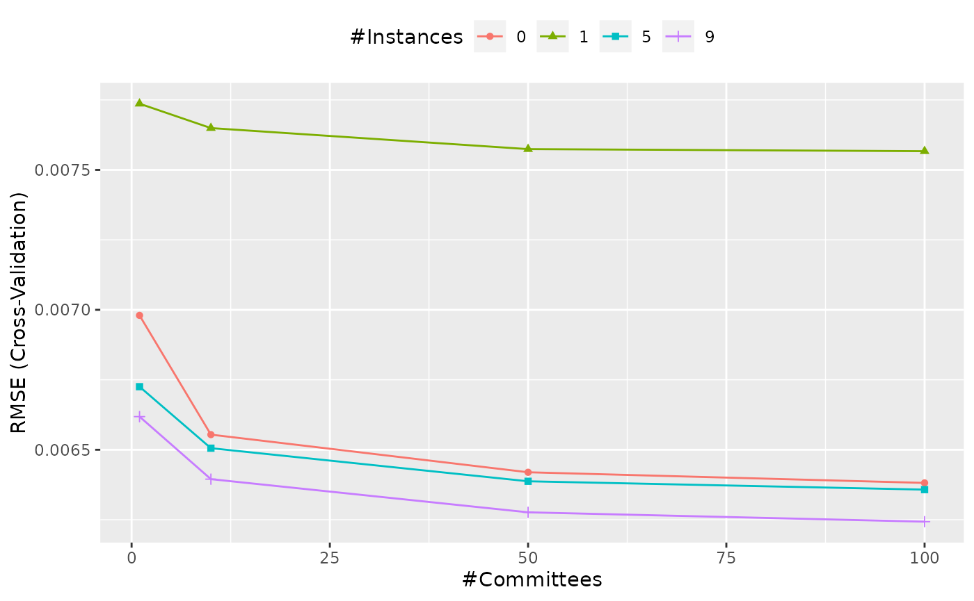
The caret_grid object selected and fit the final model
(with the best results). The test data are predicted using:
## [1] 0.7239910 0.7271985 0.7235518 0.7224333 0.7280025 0.7244288Model Tuning via tidymodels
The tidymodels packages have a slightly different approach to package
development. Whereas caret contains a large number of
functions, tidymodels splits the code into small packages that do a few
common tasks (e.g. resampling, performance estimation). To start, load
the tidymodels package and this will attach the main set of
core packages:
## ── Attaching packages ────────────────────────────────────── tidymodels 1.4.1 ──## ✔ broom 1.0.12 ✔ rsample 1.3.2
## ✔ dials 1.4.2 ✔ tailor 0.1.0
## ✔ dplyr 1.2.0 ✔ tidyr 1.3.2
## ✔ infer 1.1.0 ✔ tune 2.0.1
## ✔ modeldata 1.5.1 ✔ workflows 1.3.0
## ✔ parsnip 1.4.1 ✔ workflowsets 1.1.1
## ✔ purrr 1.2.1 ✔ yardstick 1.3.2
## ✔ recipes 1.3.1## ── Conflicts ───────────────────────────────────────── tidymodels_conflicts() ──
## ✖ rsample::calibration() masks caret::calibration()
## ✖ purrr::discard() masks scales::discard()
## ✖ dplyr::filter() masks stats::filter()
## ✖ dplyr::lag() masks stats::lag()
## ✖ purrr::lift() masks caret::lift()
## ✖ yardstick::precision() masks caret::precision()
## ✖ yardstick::recall() masks caret::recall()
## ✖ yardstick::sensitivity() masks caret::sensitivity()
## ✖ yardstick::specificity() masks caret::specificity()
## ✖ recipes::step() masks stats::step()tidymodels_prefer() resolves the naming conflicts
between it and caret functions. For example, invoking
sensitivity will now point towards the tidymodels version
(but the other function can be used via
caret::sensitivity()).
If you are new to tidymodels, we suggest taking a look at tidymodels.org or
the book Tidy Modeling with
R.
We’ll split the data into training and test data sets, then use the
vfold_cv() function to create cross-validation folds. There
are stored in a tibble object( basically a data frame):
set.seed(3)
split <- initial_split(ames, strata = Sale_Price)
tm_train <- training(split)
tm_test  <- testing(split)

set.seed(4)
cv_folds <- vfold_cv(tm_train, strata = Sale_Price)
cv_folds
## # 10-fold cross-validation using stratification
## # A tibble: 10 × 2
## splits id
## <list> <chr>
## 1 <split [1976/221]> Fold01
## 2 <split [1976/221]> Fold02
## 3 <split [1976/221]> Fold03
## 4 <split [1976/221]> Fold04
## 5 <split [1977/220]> Fold05
## 6 <split [1977/220]> Fold06
## 7 <split [1978/219]> Fold07
## 8 <split [1978/219]> Fold08
## 9 <split [1979/218]> Fold09
## 10 <split [1980/217]> Fold10To use this model, we define the model specification object
and tag which parameters that we want to tune for this model (with a
value of tune()). the package that contains the model
functions for rule-based models is called rules; we load
that first.
library(rules)

cubist_spec <-
  cubist_rules(committees = tune(), neighbors = tune()) %>%
  set_engine("Cubist")
cubist_spec
## Cubist Model Specification (regression)
##
## Main Arguments:
## committees = tune()
## neighbors = tune()
##
## Computational engine: CubistNow we can use the tune_grid() function to estimate
performance for all of the parameters in the grid data
frame:
tm_grid <-
  cubist_spec %>%
  tune_grid(Sale_Price ~ ., resamples = cv_folds, grid = grid)
tm_grid
## # Tuning results
## # 10-fold cross-validation using stratification
## # A tibble: 10 × 4
## splits id .metrics .notes
## <list> <chr> <list> <list>
## 1 <split [1976/221]> Fold01 <tibble [32 × 6]> <tibble [0 × 4]>
## 2 <split [1976/221]> Fold02 <tibble [32 × 6]> <tibble [0 × 4]>
## 3 <split [1976/221]> Fold03 <tibble [32 × 6]> <tibble [0 × 4]>
## 4 <split [1976/221]> Fold04 <tibble [32 × 6]> <tibble [0 × 4]>
## 5 <split [1977/220]> Fold05 <tibble [32 × 6]> <tibble [0 × 4]>
## 6 <split [1977/220]> Fold06 <tibble [32 × 6]> <tibble [0 × 4]>
## 7 <split [1978/219]> Fold07 <tibble [32 × 6]> <tibble [0 × 4]>
## 8 <split [1978/219]> Fold08 <tibble [32 × 6]> <tibble [0 × 4]>
## 9 <split [1979/218]> Fold09 <tibble [32 × 6]> <tibble [0 × 4]>
## 10 <split [1980/217]> Fold10 <tibble [32 × 6]> <tibble [0 × 4]>The results can be sown as a table or a plot:
collect_metrics(tm_grid)## # A tibble: 32 × 8
## committees neighbors .metric .estimator mean n std_err .config
## <dbl> <dbl> <chr> <chr> <dbl> <int> <dbl> <chr>
## 1 1 0 rmse standard 0.00700 10 0.000425 pre0_mod01_po…
## 2 1 0 rsq standard 0.778 10 0.0224 pre0_mod01_po…
## 3 1 1 rmse standard 0.00776 10 0.000404 pre0_mod02_po…
## 4 1 1 rsq standard 0.744 10 0.0202 pre0_mod02_po…
## 5 1 5 rmse standard 0.00668 10 0.000403 pre0_mod03_po…
## 6 1 5 rsq standard 0.799 10 0.0210 pre0_mod03_po…
## 7 1 9 rmse standard 0.00666 10 0.000410 pre0_mod04_po…
## 8 1 9 rsq standard 0.800 10 0.0213 pre0_mod04_po…
## 9 10 0 rmse standard 0.00625 10 0.000371 pre0_mod05_po…
## 10 10 0 rsq standard 0.823 10 0.0198 pre0_mod05_po…
## # ℹ 22 more rows
autoplot(tm_grid, metric = "rmse")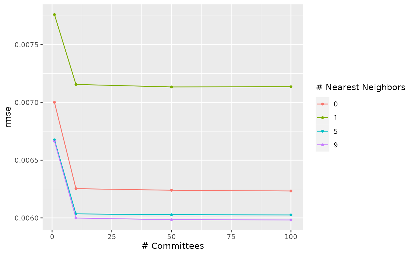
We can select a parameter combination as the final configuration and update our model specification object with those values.
cubist_fit <-
  cubist_spec %>%
  finalize_model(select_best(tm_grid, metric = "rmse")) %>%
  fit(Sale_Price ~ ., data = tm_train)

predict(cubist_fit, head(tm_test))
## # A tibble: 6 × 1
## .pred
## <dbl>
## 1 0.723
## 2 0.725
## 3 0.720
## 4 0.759
## 5 0.744
## 6 0.729This can be more easily done with last_fit():
cubist_results <-
  cubist_spec %>%
  finalize_model(select_best(tm_grid, metric = "rmse")) %>%
  last_fit(Sale_Price ~ ., split = split)

cubist_results
## # Resampling results
## # Manual resampling
## # A tibble: 1 × 6
## splits id .metrics .notes .predictions .workflow
## <list> <chr> <list> <list> <list> <list>
## 1 <split [2197/733]> train/test split <tibble> <tibble> <tibble> <workflow>
# test set results:
collect_metrics(cubist_results)
## # A tibble: 2 × 4
## .metric .estimator .estimate .config
## <chr> <chr> <dbl> <chr>
## 1 rmse standard 0.00576 pre0_mod0_post0
## 2 rsq standard 0.857 pre0_mod0_post0
# test set predictions:
collect_predictions(cubist_results)
## # A tibble: 733 × 5
## .pred id Sale_Price .row .config
## <dbl> <chr> <dbl> <int> <chr>
## 1 0.723 train/test split 0.723 5 pre0_mod0_post0
## 2 0.725 train/test split 0.722 10 pre0_mod0_post0
## 3 0.720 train/test split 0.720 11 pre0_mod0_post0
## 4 0.760 train/test split 0.758 16 pre0_mod0_post0
## 5 0.744 train/test split 0.748 18 pre0_mod0_post0
## 6 0.730 train/test split 0.726 20 pre0_mod0_post0
## 7 0.726 train/test split 0.727 23 pre0_mod0_post0
## 8 0.708 train/test split 0.708 27 pre0_mod0_post0
## 9 0.712 train/test split 0.714 34 pre0_mod0_post0
## 10 0.744 train/test split 0.746 37 pre0_mod0_post0
## # ℹ 723 more rows